Introduction to source reconstruction

To transform the electrical signals recorded on the EEG into the source space (i.e., to estimate where in the brain they originated), we first need to understand how brain activity generates signals measurable at the scalp. This is known as the forward problem in EEG. The first step is to define how neural sources are represented. The best current approximation models each source as an electric dipole — a pair of equal and opposite charges separated by a very small distance. Because of this structure, a dipole has both a magnitude (strength) and a direction, and can therefore be represented as a vector.

This dipole model is based on the properties of pyramidal neurons, which are long, oriented cells in the cerebral cortex. When many of these neurons are active and aligned, their combined electrical fields produce measurable EEG signals. Thus, the dipole serves as a simplified but biologically grounded model of how neuronal populations contribute to scalp potentials.

In the diagram below, adapted from (Grech et al., 2008), a simplification of the forward problem is shown.

Schematic three-layer head model (scalp, skull, brain) with a single dipole at position r_dip_i and one measurement electrode at r. Dipole orientation decomposed into x and z axes. — Diagram adapted from Grech et al., 2008. A three-layer approximation of the head (scalp, skull, brain) is shown with a single dipole located at position $ \mathbf{r}_{\text{dip}_i} $ from the origin. In this two-dimensional plane, any dipole orientation at that location can be decomposed into two orthogonal axes, $ \mathbf{e}_{\text{x}} $ and $ \mathbf{e}_{\text{z}} $. For simplicity, one measurement electrode $ \mathbf{m}_{\text{r}} $ is drawn at radius $ \mathbf{r} $.

The source space can be represented in one of two main ways. In a volumetric model, dipoles oriented along the x, y, and z axes are placed at discrete points throughout the whole brain volume. Alternatively, sources can be restricted to the cortical surface, where dipoles are oriented perpendicular (normal) to the cortex. This approach reduces the number of parameters to estimate and reflects the organisation of cortical pyramidal neurons.

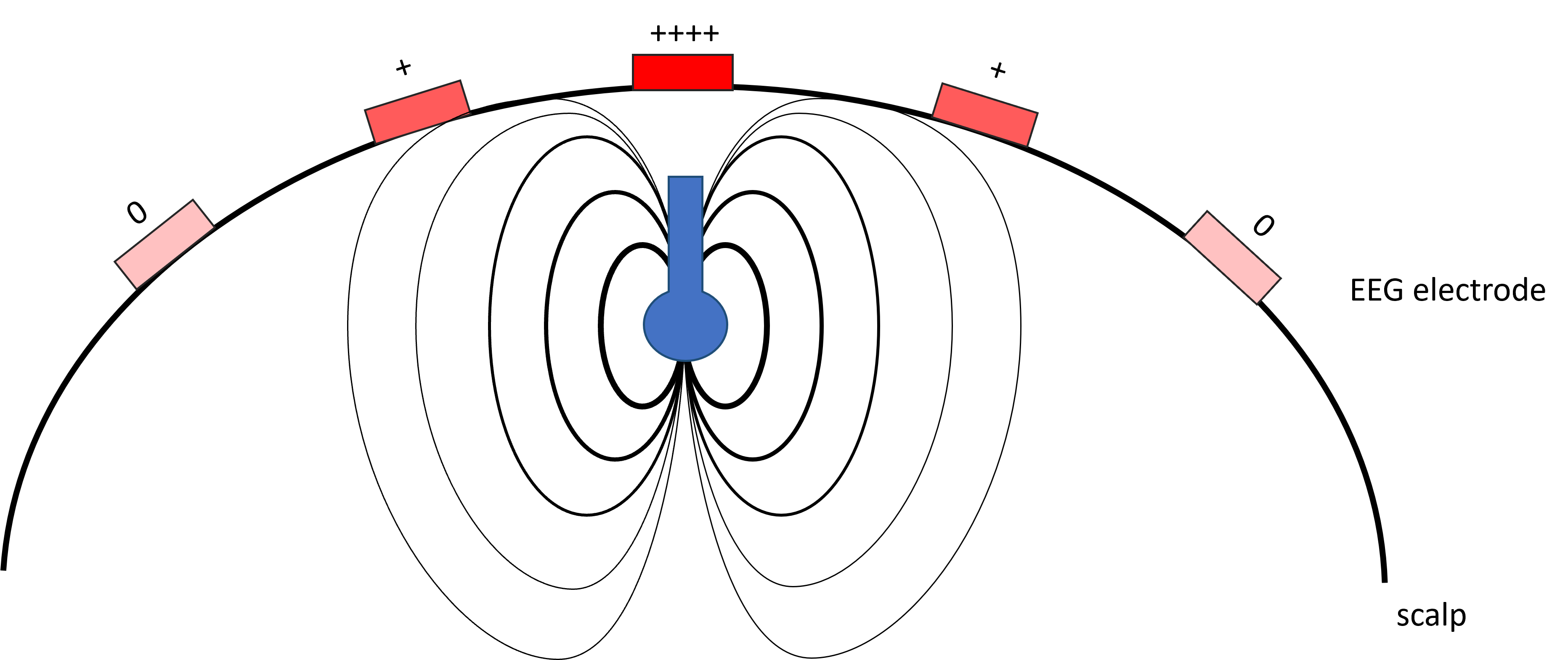
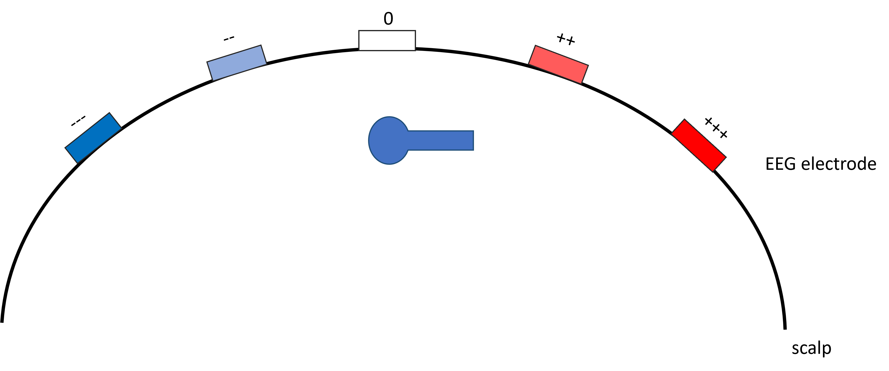
By solving the Poisson equation—using the tissues’ electrical conductivities, geometry, source locations, and EEG electrode positions as inputs—we can estimate how each dipole influences each electrode. Two examples of dipoles and their influence on the EEG electrodes are given below

Normal dipole — The electric field and influence on EEG electrodes for a normal oriented dipole

Tangential dipole — The electric field and influence on EEG electrodes for a tangential oriented dipole

According to the principle of superposition, the EEG signal measured at electrode $ m $ at time $ t $ can be expressed as a linear combination of dipole contributions, each weighted by a gain factor $ g $. All gain factors can be collected into an $ M \times N $ matrix, where $ M $ is the number of electrodes and $ N $ is the number of sources. Typically, $ M \ll N $, making the system underdetermined; in practice, $ M $ ranges from roughly 20 to 256 electrodes, whereas $ N $ is on the order of several thousand potential sources. $$ \mathbf{M} = \begin{bmatrix} m(\mathbf{r}_1) \\ \vdots \\ m(\mathbf{r}_N) \end{bmatrix} = \begin{bmatrix} g(\mathbf{r}_1, \mathbf{r}_{\text{dip}_1}) & \cdots & g(\mathbf{r}_1, \mathbf{r}_{\text{dip}_p}) \\ \vdots & \ddots & \vdots \\ g(\mathbf{r}_N, \mathbf{r}_{\text{dip}_1}) & \cdots & g(\mathbf{r}_N, \mathbf{r}_{\text{dip}_p}) \end{bmatrix} \begin{bmatrix} d_1 \mathbf{e}_1 \\ \vdots \\ d_p \mathbf{e}_p \end{bmatrix} $$

Or in compact notation, with added gaussian noise from the amplifying system $ n \sim \mathcal{N}(0,\sigma^{2}) $ $$M = GD+n$$

Below is an interactive leadfield visualisation. Use the Brain Source slider to change the source location, adjust its orientation (X, Y, Z, or custom), and explore how these parameters shape the resulting EEG scalp topography. For the full page demo click here.

Inverse Models

Distributed Source Model

Whereas dipole fitting explains the data using a few focal generators, distributed source models take the complementary approach of estimating activity at all possible source locations at once. Because the inverse problem is underdetermined or ill-posed (many candidate sources vs. relatively few sensors), the leadfield matrix $ G$ cannot be directly inverted. For a given scalp distribution $ M$, there are infinitely many source solutions $ D$. Choosing a type of inverse method is therefore equivalent to imposing a constraint that selects one solution from this solution set.

The Minimum Norm Estimate Solution

A common constraint is to choose the solution with minimal overall source power. This leads to the family of Minimum Norm Estimates (MNE).

The Tikhonov-regularised minimum-norm objective is

\[ \min_D \; \| M - G D \|_2^2 + \lambda \| D \|_2^2, \qquad \lambda>0, \]

whose stationary condition gives the familiar closed-form estimate

\[ \boxed{D_{\mathrm{MNE}} = (G^\top G + \lambda I)^{-1} G^\top M} \]

We often separate the linear operator (the inverse “filter”) from the data by writing

\[ \boxed{D_{\mathrm{MNE}} = W_{\mathrm{MNE}} \; M, \qquad W_{\mathrm{MNE}} = (G^\top G + \lambda I)^{-1} G^\top.} \]

Two practical observations about this form: (1) the operator $W_{\mathrm{MNE}}$ does not depend on the data $M$ and can therefore be precomputed; (2) the direct form above requires inverting an $N×N$ matrix (number of sources), which may be computationally expensive.

The generalised MNE expresses prior knowledge about source amplitudes through a source covariance (or prior) matrix $R$. With this prior the operator becomes

\[ \boxed{ W_{\mathrm{MNE}} \;=\; R\, G^\top \big( G\,R\,G^\top + \lambda I \big)^{-1} } \]

and the estimate is

\[ \boxed{ D_{\mathrm{MNE}} = W_{\mathrm{MNE}} \; M \;=\; R\,G^\top \big( G\,R\,G^\top + \lambda I \big)^{-1} M }. \]

When the prior is the identity, $R = I$, the generalised operator reduces to the usual MNE operator:

\[ R = I \quad\Rightarrow\quad W_{\mathrm{MNE}}^{(R)} = G^\top \big( G G^\top + \lambda I \big)^{-1}. \]

The advantage of the generalised form is twofold: (i) an informative source prior $R$ (e.g., encoding expected variance, orientation constraints, or spatial covariances) is incorporated naturally; (ii) the computation typically involves inversion of an M×M matrix (number of sensors) rather than an N×N matrix when implemented via the latter expression, which is computationally preferable in typical EEG/MEG setups.

Inherently, this solution is biased towards shallower sources, since sources closer to the measurement electrodes require less amplitude to give a similar signal with respect to deeper sources. A common practical correction for depth bias is to include a diagonal depth-weighting matrix $W_{\mathrm{depth}}$ (not to be confused with the operator $W$). One way to incorporate depth weighting into the generalised framework is to absorb it into the source prior:

\[ R \leftarrow W_{\text{depth}}^{-2} \quad\text{(i.e., use a prior variance that compensates for smaller lead-field norms).} \]

Alternatively, the weighted Tikhonov objective

\[ \min_D \; \| M - G D \|_2^2 + \lambda \| W_{\text{depth}} D \|_2^2 \]

yields the equivalent explicit weighted solution

\[ \boxed{ D_{\mathrm{wMNE}} = (G^\top G + \lambda W_{\text{depth}}^\top W_{\text{depth}})^{-1} G^\top M } \]

or, using the generalised/prior viewpoint with $R = (W_{\text{depth}}^\top W_{\text{depth}})^{-1}$,

\[ \boxed{ D_{\mathrm{wMNE}} = R\,G^\top \big( G\,R\,G^\top + \lambda I \big)^{-1} M }. \]

From a general point of view, any prior on the sources which can be summarised in an operator $B$ as:

\[ \min_D \; \| M - G D \|_2^2 + \lambda \| BD \|_2^2 \]

yields the explicit solution

\[ \boxed{ W_{\mathrm{wMNE}} = (G^\top G + \lambda B^\top B )^{-1} G^\top} \]

or, using the generalised/prior viewpoint with $R = (B^\top B)^{-1}$.

One classical prior is spatial smoothness.

LORETA and LAURA — MNE solution with spatial priors

LORETA and LAURA can be seen as MNE solutions where the regulariser encodes spatial priors.

LORETA (low resolution brain electromagnetic tomography) uses a discrete Laplacian operator $L$ (second-order neighborhood) that penalises rapid spatial changes. The objective is

\[\min_D \| M - G D \|_2^2 + \lambda \| LW_{\text{depth}} D \|_2^2\]

giving

\[\boxed{ W_{\mathrm{LORETA}} = (G^\top G + \lambda (LW_{\text{depth}})^\top LW_{\text{depth}})^{-1} G^\top}\]

or, using the generalised/prior viewpoint with $R = ((LW_{\text{depth}})^\top LW_{\text{depth}})^{-1} = (W_{\text{depth}}^\top L^\top L W_{\text{depth}})^{-1}$

This yields the smoothest possible solution.

LAURA (Local Auto-Regressive Averages) replaces the Laplacian with a flexible, distance-weighted prior matrix

The choice of spatial prior controls smoothness scale and effective spatial resolution.

Normalised methods: dSPM, sLORETA and eLORETA

To reduce the influence of noise and improve statistical interpretability or remove localisation bias, MNE-type estimates are often normalised at each source voxel.

dSPM (dynamic statistical parametric mapping)

dSPM normalises the MNE estimate by the (estimated) standard deviation of the noise at each source:

\[ D_{\mathrm{dSPM}} = W_{\mathrm{dSPM}} \; D_{\mathrm{MNE}} , \quad W_{\mathrm{dSPM}} = \operatorname{diag}\Big( \sqrt{\operatorname{diag}\big( W_{\mathrm{MNE}} C_n W_{\mathrm{MNE}}^\top \big)} \Big)^{-1} \]

Here $C_n$ is the noise covariance matrix estimated from baseline or empty-room recordings. The result is a z-like map where each source value is scaled by its noise standard deviation.

sLORETA (standardized LORETA)

sLORETA applies a standardisation to the MNE estimator such that, under ideal conditions, the localisation bias is eliminated:

\[ D_{\mathrm{sLORETA}} = \left( \operatorname{diag}\big( R_{\mathrm{WME}} \big) \right)^{-1/2} \; D_{\mathrm{MNE}} , \quad \text{with } R_{\mathrm{WME}} = W_{\mathrm{WME}}G \quad \text{the resolution matrix.}\]

eLORETA (exact LORETA)

eLORETA is a variant of sLORETA, where the normalisation to eliminate the localisation bias is done by an interative re-weighting process.

Beamformers (spatial filters)

Distributed methods estimate the contribution of many small sources simultaneously.Beamformers compute a linear spatial filter that enhances activity originating from a target source location while suppressing contributions from all other locations. The filter weights depend on both the leadfield at the target location and the data covariance matrix, making beamformers intrinsically data-adaptive.

LCMV Beamformer

The classical Linearly Constrained Minimum Variance (LCMV) beamformer finds spatial weights that (i) pass activity from the target source with unit gain, while (ii) minimising the projected power of all other sources and noise.

The optimisation problem is

\[ \min_w \; w^\top C \, w \quad \text{subject to} \quad w^\top g = 1, \]

where $C$ is the data covariance matrix and $g$ is the leadfield vector for the target source (i.e., the column of $G(.,i) = g$ ).

The resulting weight vector is

\[ \boxed{ w_{\mathrm{LCMV}} = \frac{C^{-1} g}{g^\top C^{-1} g} } \]

The estimated source activity at that location is then obtained by projecting the sensor data $M$ through the beamformer:

\[ \hat{D}(r) = w_{\mathrm{LCMV}}^\top M. \]

One can see that the spatial filter $w_{\mathrm{LCMV}}$ is dependent on the data but independent of the other estimated sources of interest. These are key differences with distributed source model.

Because leadfield strength decreases with source depth, unit-gain beamformers assign larger weights to deep sources, which in turn inflates their estimated power. This center-of-head bias prevents direct comparisons of power across space. Normalised beamformer variants, such as array-gain normalisation, address this issue by correcting the filter sensitivity.

Array Gain Normalisation

Array gain normalisation compensates the center-of-head bias by scaling the beamformer weights such that the filter's sensitivity is equalised across all candidate locations.

The array gain LCMV at a location with weight vector $w$ and leadfield $g$ is defined as

\[ \min_w \; w^\top C \, w \quad \text{subject to} \quad w^\top g = \|g\|, \]

Using the unit-gain LCMV formulation,

\[ \boxed{ w_{\mathrm{LCMV, array\text{-}gain}} = \frac{C^{-1} g_n}{{g_n}^\top C^{-1} g_n}, \quad \text{with} \quad g_n = \frac{g}{\|g\|}} \]

The estimated activity then becomes

\[ \hat{D}_{\mathrm{norm}}(r) = \left( w_{\mathrm{LCMV}}^{\mathrm{gain\text{-}norm}} \right)^\top M, \]

ensuring that differences in estimated activity reflect neural effects rather than purely spatial variations in beamformer sensitivity. For more details on beamformer we recommend this paper: Westner et al., 2022.